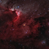
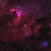
The Cave Nebula, Sh2-155 or Caldwell 9, is a dim and very diffuse bright nebula within a larger nebula complex containing emission, reflection, and dark nebulosity. It is located in the constellation Cepheus. The dark nebula complex to the right is designated LDN 1216. There is also one reflection nebula, VdB 155, in the bottom right corner - just next to LDN1216. About 2,400 light-years away, the scene lies along the plane of our Milky Way Galaxy toward the royal northern constellation of Cepheus. Astronomical explorations of the region reveal that it has formed at the boundary of the massive Cepheus B molecular cloud and the hot, young, blue stars of the Cepheus OB 3 association. The bright rim of ionized hydrogen gas is energized by the radiation from the hot stars, dominated by the bright blue O-type star above picture center. Radiation driven ionization fronts are likely triggering collapsing cores and new star formation within. Appropriately sized for a stellar nursery, the cosmic cave is over 10 light-years across.
This time I set out to do something a bit new. I knew that the field of view would contain a reflection nebula (VdB 155) which would not pick up easily using narrow band filters. Thus I, in addition to narrow band images also shot one image using a blue filter. Since my observatory is drenched in heavy light pollution I needed a lot of photons, which I achieved by binning 3x3. I also shot all narrow band images binned 1x1 - instead of my normal 3x3 binning. This meant I had to take more OIII and SII subs. This made it possible for me to make a new type of artificial RGB combination of the data. I normally stretch Ha, OIII and SII so that their histograms match. This is exactly what one shall do for a Hubble combination, but for an artificial RGB combination the OIII (and SII) contribution will be too large, resulting in an image with "whitish" areas (frist image in the second row of thumbnails). I usually compensate by dailing down the OIII contribution to get a "redder" image (second image in the second row of thumbnails). The problem with having different binnings (1x1 for Ha and 3x3 for SII and OIII) is that the relative strength is a bit difficult to adjust for. In a four hour bin 3x3 image each pixel has recieved nine times as many photons compared to a four hour bin 1x1 image. Having all images at bin 1x1 made it easier to relate the strengths of three narrow band images. In the third row, first image, I just gave all narrow band images the same stretch and combined them according to a recipie (see below) to give an approximation to a "normal" RGB image. It is good to see how close that image is to the one using my old (somewhat faulty) technique. To that image I could now add the blue image to make the reflection nebula come forward (thrid row, second image).
Mouseover of the small thumbnails to the left will show the six different combinations of three narrowband images (Ha, OIII and SII).
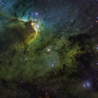
Hubble Standard: R = SII, G = Ha, B = OIII. The first thumbnail in the first row is the familiar Hubble composition where the Ha, OIII and SII images has been adjusted so that they all have similar histograms. In this way the OIII and SII contribution will show up. If this histogram equalization is not done, the image will be dominated by the Ha channel, i.e. it will be green.
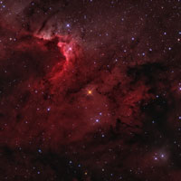
Hubble colour shift: The second thumbnail in the first row is based on the top-left, to which a colour shift has been applied Photoshop's Selective Color tool (see Bob Frankes tutorial). One has to be very careful when using the Selective Color tool in PS, since it is easy to shift to much resulting in sharp borders between colours.
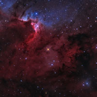
Hubble modified: The third thumbnail in the first row is a modification to the Hubble composition (Orange = Ha (hue=35), Red = SII (hue=0), Cyan = OIII (hue=210). Instead of assigning Ha to green I assigned Ha to orange (Hue = 35 in PS notation), SII to red (as in Hubble) and OIII to a slightly more turquoise hue (Hue = 210 in PS notation). This palette has the advantage of separating the different narrowband images (as do the Hubble colour shifting composition), but has the advantage of not being dependent on careful usage of the Selective Color tool.
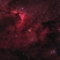
Artificial RGB from Hubble images: The first thumbnail in the second row is an attempt at mapping the narrowband images, used in the Hubble image, to colours (R = 80%Ha + 20%SII, G = OIII, B = 85%OIII + 15%Ha) so that the image would mimic the result of a broadband RGB image. It has been constructed by using the fact that H-beta emission (blue) accompanies the H-alpha line (red) with H-beta roughly 15% of the strength of the H-alpha. To the best of my knowledge this was first suggested by Richard Crisp. It also uses the fact that OIII is positioned in-between the blue and green part of the spectra. A litte bit of SII is added to the red channel.
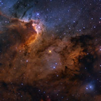
ARGB redder from Hubble images: the second thumbnail in the second row is based on the Artificial RGB image described above but the OIII contribution has been dialled down. Sometimes the ARGB blend above gives white areas where OIII is the strongest. In order to get a more "realistic" RGB representation the OIII contribution to both the blue and the green channel can be turned down to your subjective liking.
ARGB bluer from Hubble images: the third thumbnail in the second row is based on the Artificial RGB image described above but the OIII contribution to the blue channels has been dialled up. One of the ideas behind the Hubble palette representation is that it visualizes the different contributions Ha, OIII, SII. This can also be achieved in a RGB like representation by dialling up the OIII contribution to the blue channel. In this way the OIII areas will be bluish, the Ha areas will be reddish and the SII areas will be deep red.
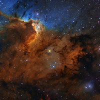
Artificial RGB: The first thumbnail in the thrid row is an attempt at mapping the narrowband images to colours (R = 80%Ha + 20%SII, G = OIII, B = 85%OIII + 15%Ha) so that the image would mimic the result of a broadband RGB image, using narrow band images with the same stretch. It has been constructed by using the fact that H-beta emission (blue) accompanies the H-alpha line (red) with H-beta roughly 15% of the strength of the H-alpha. To the best of my knowledge this was first suggested by Richard Crisp. It also uses the fact that OIII is positioned in-between the blue and green part of the spectra. A litte bit of SII is added to the red channel.
Artificial RGB with reflection nebula: The same as Artificial RGB above to which the blue image has been added to show the reflection nebula.
In order to make most use of the weak OIII and SII data I have also used JP Metsavainio's Tone Mapping technique. A pdf that outlines tone mapping can be found here, and in order to bring out as much details as possible I have followed some of the tutorials on Ken Crawford's site.
Below you see images for each emission line respectively. The images has been stacked and stretched the same amount.
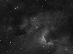
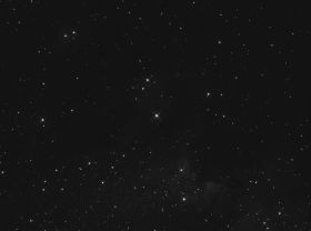
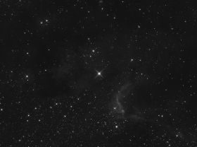
Ha OIII SII
The following software has been used. CCDAutoPilot5 (for control), MaximDL (image acquisition and guiding), CCDStack (calibration and RGB scaling, PixInsight (cropping, background correction, colour corrections) and Photoshop CS5 (all the rest, incl Noel Carbonis Astronomy Tools), and finally JP Metsavainio's Tone Mapping technique.
This image was processed in December 2013